Chapter 3 Week 3
3.1 Preliminary infomation
3.1.1 Presentation of units on tables and graphs
Your tables should have units expressed in the column headers where appropriate, and uncertainties should be expressed in the header if they are constant across the whole range, or in parentheses for each measurement if different. Units should be expressed as “Quantity / unit” to allow you to express them as dimensionless quantities in the table or on the axis of your graph (please note brackets are absolutely incorrect).
This is because this is how our governing body (IUPAC) tell us how to do it. See the IUPAC Green Book (2012 edition, page 3).
You can think of the horizontal line below the header as an equals sign, so:
| [KI] / M | [KNO2] / M | Emission intensity / 103 cps | τ / ns |
|---|---|---|---|
| 0 | 1.100 | 16.580 | 17.60 |
| 0.040 | 1.060 | 3.753 | 3.90 |
| 0.100 | 1.000 | 1.566 | 1.80 |
| 0.200 | 0.900 | 0.721 | 0.95 |
| 0.300 | 0.800 | 0.446 | 0.64 |
| 0.500 | 0.600 | 0.242 | 0.39 |
| 0.800 | 0.300 | 0.121 | 0.25 |
in the table above the third value down in the first column can be expressed as:
[KI] / M = 0.100
which of course rearranges to:
[KI] = 0.100 M.
If we look at the top value in the third column:
Emission intensity / 103 cps = 16.580
which of course rearranges to:
Emission intensity = 16.580 × 10³ cps
3.1.2 Plotting of graphs
When ever we plot a graph we have to determine what we plot on each of the two axes.
The independent variable is the variable we have control over, we plot it (or something related to it) on the x-axis (the horizontal axis).
The dependent variable is the varible we measure, we plot it (or something related to it) on the y-axis (the vertical axis).
These axis should under most circumstances not contain constants unless those constants are specific to the experiment.
There is no need to start a graph axis at zero - you do not need a ‘squiggle’ on the axis to show that it is not starting at zero (that is what the numbers on the axis tell you), this squiggle (or more formally an axis break) does have a job when plotting graphs, but usually the use by first year undergraduates is incorrect.
When plotting a graph, we want to have broken down the equation we are using to fit the linear relationship:
\[\begin{equation} y = mx+c \tag{3.1} \end{equation}\]
We should never force a graph through a particular intercept (c).
It is important when we ever have performed a calculation to determine values to plot on either x or y axis that we have taken account for any multipliers in the header, and that units ar SI (such as tempeature in K!).
A gradient is calculated by determining the change in y divided by the change in x:
\(m= \frac{\Delta y}{\Delta x}\)
Don’t forget units on gradients! The units of a gradient are the units on y divided by the units on x.
Usually graphs are now drawn on a computer, we teach you how to draw graphs in both Excel (figure 3.1) in Key Skills, and Python (figure 3.2) in the Comp Chem labs. However it can be useful to be able to quickly draw a graph by hand as well.
Hints and tips for drawing the perfect graph
- Data points should be plotted as a dot (not a line), and data points should not be connected by a line.
- A trendline should only be fitted if there is a mathematical reason to do so.
- Graphs should be on a plain background (no gridlines).
- Axes do not need to start at zero - you do not need that funny squiggly line if it doesn’t start at zero.
- Axes should be labeled with value and unit (if required), the unit should appear behing a solidus (/), you should not use brackets.
- If the numbers plotted are very small or very large (such that there could be confusion over the numbers on the axes) a multiplier should be included in the axes title.
- If concentration is being plotted you should use square brackets to indicate the concentration of what e.g. [azulene] / µM not concentration / µM.
- A title should normally be included, but this is a placeholder for a figure caption which you will use in later years.
- The title should include all relevant details about the graph which are not otherwise included, this may be as simple as the question number, or a full description of other experimental conditions.
3.2 Example of plotting graphs
The Stern-Volmer (Equation (2.14)) shows how the lifetime \(\tau\) of a dye changes with concentration of a quencher, [Q]. The data in Table 3.1 can be modeled using the Stern-Volmer equation, you will note that this equation uses terms with a subscript 0 (\(\tau_0\)), when values like this are frequently used in chemistry (and physics).
\[\begin{equation} \frac{\tau_0}{\tau}=1+k[Q] \tag{3.2} \end{equation}\]
where \(k = k_q \tau_0\).
These ‘subscript 0’ values are referencing values when the independant variable is zero, so \(\tau_0\) = 17.60 ns.
You will notice that Equation (2.14) is already arranged into \(y=mx+c\), where the x variable is [KI] and the y variable is \(\frac{\tau_0}{\tau}\). This means that the gradient is k, and the intercept 1.
Figures 3.1 & 3.2 show this data plotted in Excel and Python respectively, no title is included because I’ve got figure captions.
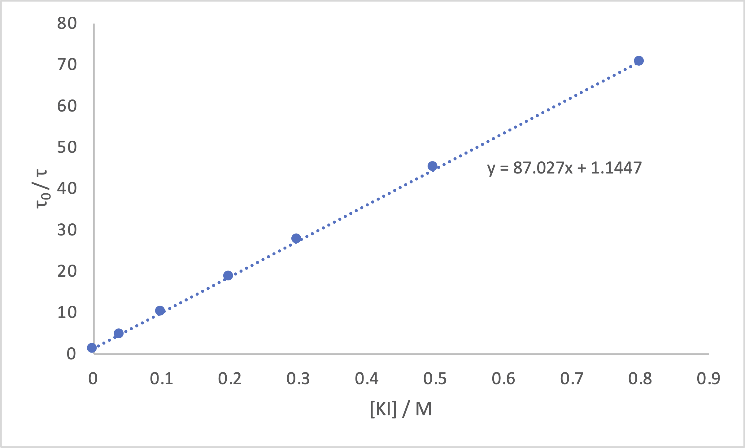
Figure 3.1: The Stern-Volmer plot from the data above drawn in excel.
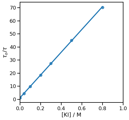
Figure 3.2: The Stern-Volmer plot from the data above drawn in python.
3.3 Summary of concepts learnt
- Units and any scaling factors should appear behind a solidus (/) not brackets.
- Tables with headers work like equations, the horizontal bar works like a equals sign.
- It should always be clear what is contained in a table - use square brackets for concentrations
- Equations should be rearranged so they can be plotted in the form \(y=mx+c\).
When plotting graphs:
- the dependent variable (the thing you have control of or something related to it) goes on the horizontal \(x\)-axis.
- the independent variable (the thing you measure or something related to it) goes on the vertical \(y\)-axis.
- when plotting data data points should be used and they should not be connected by lines.
- a line of best fit should be used when there is a mathematical reason to do so, so if plotting data as \(y=mx+c\) a straight line should be fitted.
- you should never force a line of best fit through a given intercept.
3.4 Questions
When plotting graphs feel free to plot either by hand, in python, excel or numbers. The choice is entirely up to you.
3.4.1 Sketch graphs
Answers for these questions are in Section 3.5.1.
For the following equations sketch suitable linear plots indicating values of the intercept and gradient on each sketch.
Show how absorption, \(A\), changes with concentration, \(c\): \(A = \varepsilon c l\)
Show how pressure, \(p\), changes with temperature, \(T\): \(pV = nRT\)
Show how pressure, \(p\), changes with volume, \(V\): \(pV = nRT\)
3.4.2 Second order kinetics
Answers for these questions are in Section 3.5.2.
Use the following table of data to plot a graph of \(\frac{1}{[A]}\) against t. Find the gradient and intercept.
(Just to note here you are plotting the equation \(\frac{1}{[A]}=\frac{1}{[A]_0}+kt\)).
| t / s | 104 [A] / mol dm-3 |
|---|---|
| 100 | 21.0 |
| 200 | 12.0 |
| 300 | 8.4 |
| 400 | 7.1 |
| 500 | 5.6 |
3.4.3 Clausius-Clapeyron equation
Answers for these questions are in Section 3.5.4.
The relationship between the vapour pressure and temperature of diethyl ether (Table 3.2) can be modeled using the Clausius-Claeyron equation (Equation (3.3)) to determine the enthalpy of vapourisation \(\Delta _{vap}H^\circ\).
\[\begin{equation} \ln p = -\frac{\Delta_{vap}H^\circ}{RT}+C \tag{3.3} \end{equation}\]
- Determine \(\Delta _{vap}H^\circ\).
- Determine the temperature diethyl ether boils at, at 1 atmosphere (760 mm Hg). Hint: determine C
| \(p\) / mm Hg | T / ºC |
|---|---|
| 17 | -38 |
| 28 | -30 |
| 40 | -25 |
| 55 | -20 |
| 75 | -15 |
| 97 | -10 |
| 125 | -5 |
| 157 | 0 |
3.4.4 Arrhenius equation
Answers for these questions are in Section 3.5.4.
The Arrhenius equation (Equation (2.14) shows how the rate of reaction, \(k\), depends upon the temperature of the reaction, \(T\)).
\[\begin{equation} k=Ae^{-\frac{E_a}{RT}} \tag{2.14} \end{equation}\]
For the data shown in Table 3.3 plot an appropriate linear plot in order to determine the activation energy, \(E_a\), and the pre-exponential factor, \(A\).
| T / ºC | k / 105 s-1 |
|---|---|
| 283 | 0.000352 |
| 356 | 0.0302 |
| 393 | 0.219 |
| 427 | 1.16 |
| 508 | 39.5 |
3.5 Answers
3.5.1 Sketch graphs
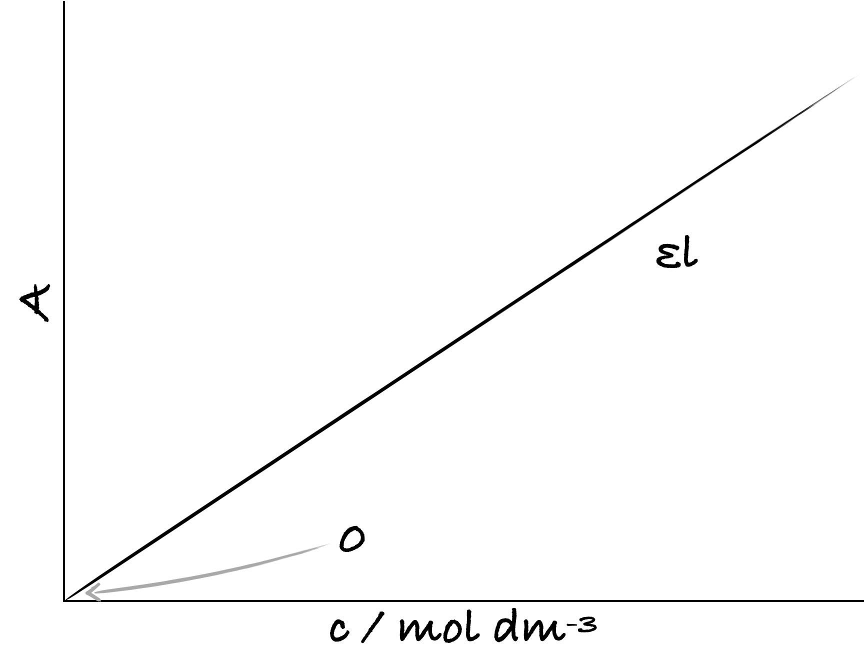
Figure 3.3: The Beer-Lambert relationship to show how absorbance, the dependent variable, changes with concentration, the independent variable.
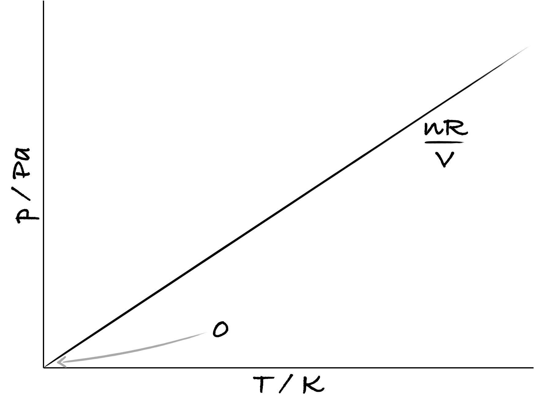
Figure 3.4: A sketch to show how the pressure of an ideal gas, the dependent variable,changes with temperature, the independent variable.
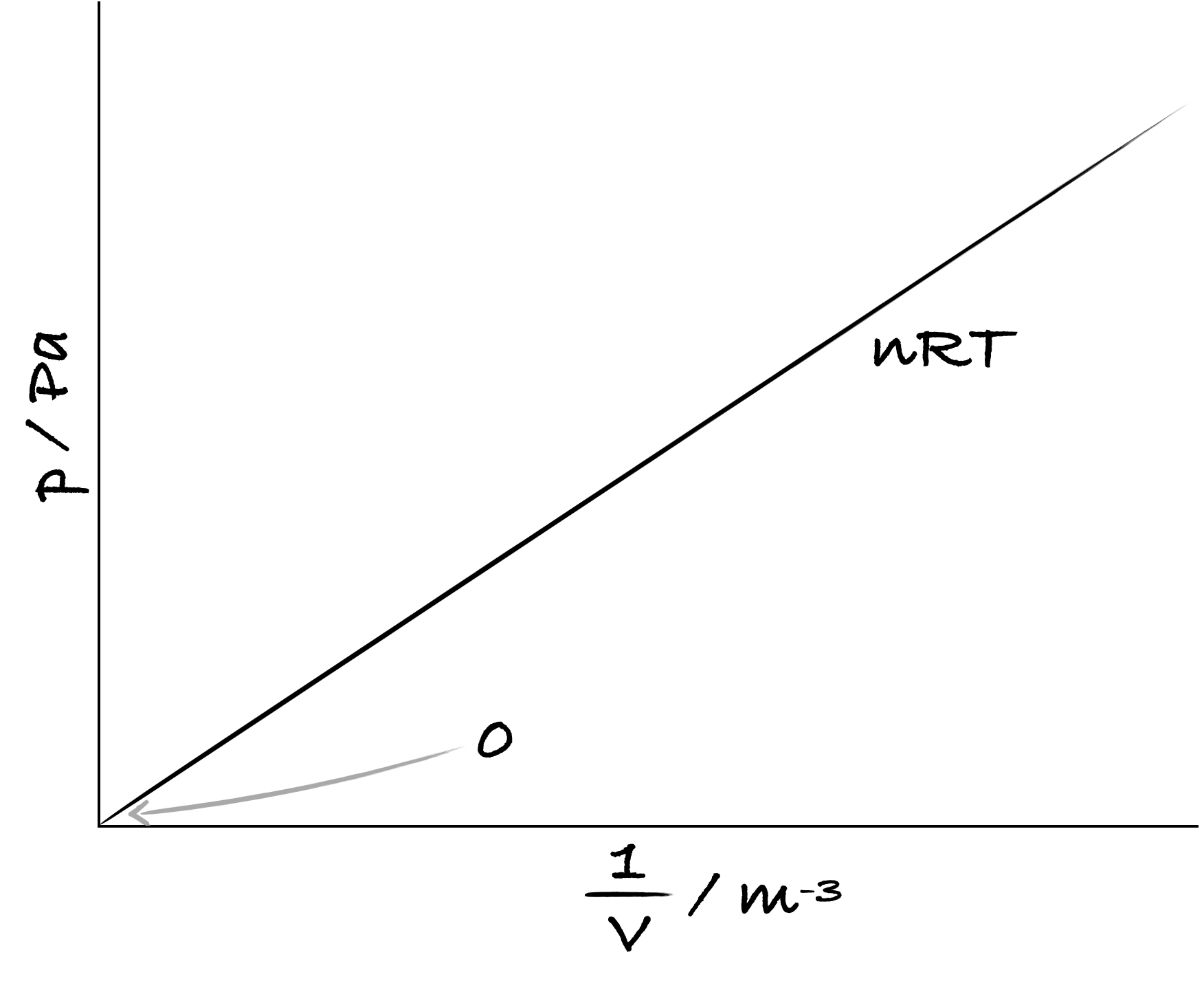
Figure 3.5: A sketch to show how the pressure of an ideal gas, the dependent variable,changes with volume, the independent variable - note for a linear relationship we have 1/V on the x-axis.